Chapter 5 — Production Possibility Curves
Cambridge International AS & A Level Economics (9708) · Unit 1.5 · 4th edition coursebook
Learning objectives
- Explain the meaning and purpose of a production possibility curve.
- Explain the shape of the production possibility curve, including the difference between constant opportunity costs and increasing opportunity costs.
- Analyse the causes and consequences of shifts in a production possibility curve.
- Discuss the significance of a position within a production possibility curve.
Key terms
- production possibility curve (PPC)
- A simple representation of the maximum level of output that an economy can achieve, given its current resources and state of technology; may be referred to as a production possibility frontier.
- trade-off
- What is involved in deciding whether to give up one good for another good.
- productive capacity
- The maximum output that can be produced when all resources are used fully.
5.1The production possibility curve
What an economy can produce is determined by the quantity and quality of the factors of production it has available. High-income economies have a wide range of factors of production and consequently produce many thousands of distinct goods and services. Low-income economies have fewer factors, and lower-quality factors, so they produce a narrower range. The set of possible output combinations an economy could produce is its production possibilities.
Economists use a simple model — the production possibility curve (PPC), sometimes called the production possibility frontier — to display these possibilities on a two-good diagram.
How the production possibility curve works
To make the model tractable, imagine an economy that produces just two goods — say, cars and televisions — and that uses all of its resources between them, at the present state of technology. The PPC then draws the boundary between what the economy can produce and what it cannot. Any point exactly on the curve represents a production situation where output is maximised. Figures 5.2 and 5.3 show two PPCs of different shapes.
Figure 5.4 shows the PPC for the cars-and-televisions example. The two extreme points on the curve correspond to allocating all of the economy's resources to one good or the other: every other point on the curve represents a combination of cars and televisions where the economy is using its resources fully. Each point on the curve indicates an efficient allocation of resources — the economy is getting all it can from the inputs available.
A point inside the curve — such as point C in Figure 5.4 — represents an inefficient allocation: the economy is producing less than its resources would allow. A point outside the curve — such as point D — is currently unattainable; the economy does not yet have the resources or technology required to produce that combination. This is the geometric expression of scarcity.
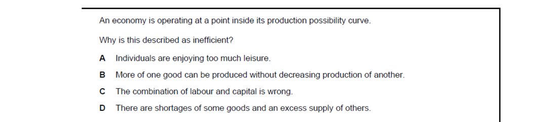
A point inside the PPC means some factors are unemployed or underused, so it is possible to raise output of one good without giving up any of the other. Option B captures this defining characteristic of productive inefficiency. Leisure (A) is not an output on the diagram, factor-mix problems (C) describe allocative inefficiency, and shortages/surpluses (D) are demand-side issues.
5.2The production possibility curve and opportunity cost
The PPC is a natural way to show opportunity cost. When the economy moves from one point on the curve to another, more of one good is being produced and less of the other. The amount of one good given up to gain more of the other is the opportunity cost of the gain.
The two PPC shapes illustrate two different opportunity-cost patterns. In Figure 5.2 (a straight-line PPC), reducing production of one good by a fixed amount always allows the same proportionate increase in the other. The opportunity cost is constant. In Figure 5.3 (a PPC bowed outwards from the origin), reducing production of one good produces a larger increase in the other when that good is being produced in small quantities, and a smaller increase when it is already being produced in large quantities. The opportunity cost is increasing.
The numerical example in Figure 5.4 makes this concrete. Moving from point A to point B reallocates resources from the car industry to the television industry. The result is fewer cars and more televisions, and the ratio between cars given up and televisions gained at that point on the curve is the opportunity cost of the additional televisions.
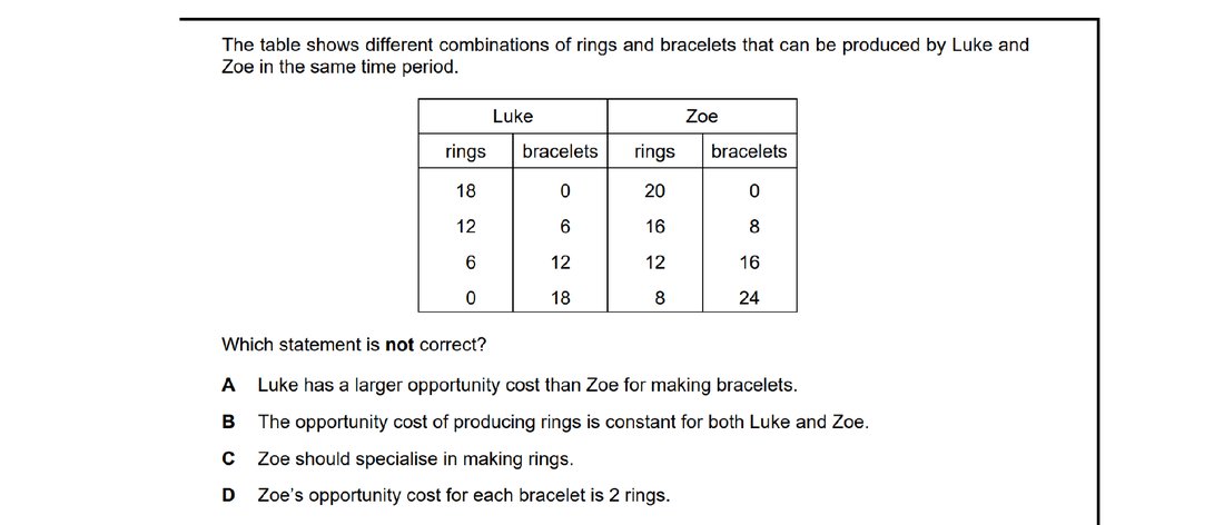
Comparative advantage and opportunity cost: from the table, Zoe gives up 24 bracelets to produce 20 rings, so each bracelet costs her 20/24 = 5/6 of a ring, not 2 rings. Option D's claim of 2 rings per bracelet is therefore incorrect. The other statements correctly describe constant opportunity costs and Zoe's lower cost of ring production, making rings her specialisation.
5.3The shape of the production possibility curve
The shape of the PPC carries information. In Figure 5.4, the curve is bowed outwards. Where the economy is allocating most of its resources to televisions, the curve is steep — additional televisions require giving up a large number of cars. Where the economy is allocating most of its resources to cars, the curve is flatter — each television given up yields only a small increase in cars. This is the geometry of increasing opportunity cost.
When the PPC is a straight line (Figure 5.2), opportunity costs do not change as the economy moves along the curve. Constant opportunity costs arise when factors of production are equally well suited to both goods — for example, when two similar products require essentially the same inputs.
When the PPC is bowed outwards (Figure 5.4), opportunity costs change as the economy moves along the curve. Producing additional units of one good progressively requires factors of production that are less and less suited to that good, raising the opportunity cost of each additional unit. This is the typical case where the two goods require materially different combinations of factors.
A trade-off between products
The PPC also shows the trade-off between products. A trade-off is the decision about whether to give up some of one good in order to obtain more of another. With resources fully employed on the curve, producing more televisions necessarily means producing fewer cars. The magnitude of the trade-off in any region of the curve is given by the slope of the curve at that point.
A change in available resources
Up to this point we have assumed that resources are fixed. In reality, technological advance steadily raises productivity, which means more output can be produced from the same resources. Where the change affects one good more than the other — for example, a major productivity gain in television production but no change in car production — the PPC pivots. Figure 5.5 shows this: the new PPC (PPC 2) reaches a higher quantity of televisions on the horizontal axis, while the vertical-axis intercept for cars stays the same. For any given quantity of cars, the economy can now produce more televisions than before.
5.4Shifts in the production possibility curve
In some situations the PPC does not just pivot but shifts in its entirety — outwards or inwards. A shift of the entire curve means the productive capacity of the economy has changed.
- An outward (rightward) shift indicates an increase in productive capacity.
- An inward (leftward) shift indicates a decrease in productive capacity.
Two main causes drive these shifts.
More resources become available. Productive capacity grows when factor inputs increase — for example, growth in the labour force through immigration, more capital goods through investment, or improved opportunities for enterprise — or when the quality of those inputs improves through education and training. The opposite is also possible: overpopulation or factor destruction can leave fewer resources available and shift the PPC inwards. Figure 5.7 shows both directions.
Technological change. Technology advances over time and these advances usually shift the PPC outwards: more of both goods can be produced from the same resources. In rare circumstances, technological regress (for example, a loss of accumulated know-how, or destruction of capital from war) can shift the PPC inwards.
Key concept link — scarcity and choice
On a production possibility curve, choice is represented by any point on the curve. This indicates the many possible choices of combinations of goods when maximising the use of available resources. Scarcity is represented on the axes by the maximum possible outputs that are possible with these resources.
Key concept link — time
The simple model of a production possibility curve shows the effects of a change to the allocation of resources in the short-run and long-run periods.
Using the production possibility curve to show choices
The PPC is particularly useful in illustrating the difficult choices many low-income economies face. Figure 5.8 shows a PPC for consumer goods (horizontal axis) and capital goods (vertical axis). When most of the economy's resources are devoted to consumer goods, production sits high up on the consumer-goods axis but the resources available for capital goods are very small. New investment in capital goods is then often only enough to replace existing capital, and the economy's productive potential does not grow.
For productive potential to rise, a larger proportion of resources needs to be devoted to capital goods. A small reduction in consumer-goods output (A to B on the diagram) can produce a relatively larger increase in capital-goods output (C to D). Over time, the increased capital stock shifts the PPC outwards, generating future economic growth. The price is a short-run sacrifice of consumption to enable a long-run rise in capacity.
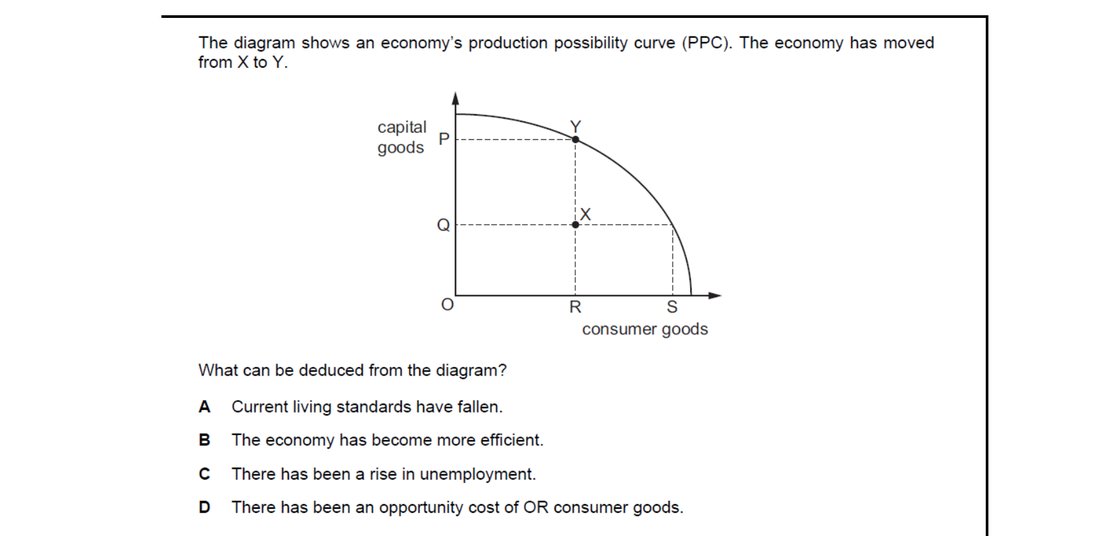
Movement from X to Y is from inside the PPC to a point on it, so the economy is now using its resources fully and without waste. Option B – the economy has become more efficient – captures this. Living standards have not fallen and unemployment has not risen (both fall as the economy reaches the frontier), and opportunity cost is measured between points on the curve, not from inside it.
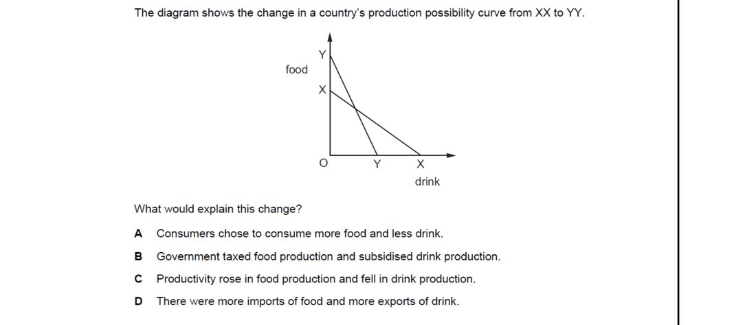
When productivity rises in one industry and falls in another, the maximum output of each changes asymmetrically — the curve pivots, expanding on the food axis and contracting on the drink axis. Option C – productivity rose in food production and fell in drink production – is the only cause that produces this asymmetric pivot. Demand or trade changes (A, D) move points on the PPC, not the curve itself; taxes (B) shift incentives, not the productive frontier.
End-of-chapter practice
Past-paper questions from CIE 9708. Pick A, B, C or D. Answers are saved on this device — press Download report (PDF) at the top to save them.
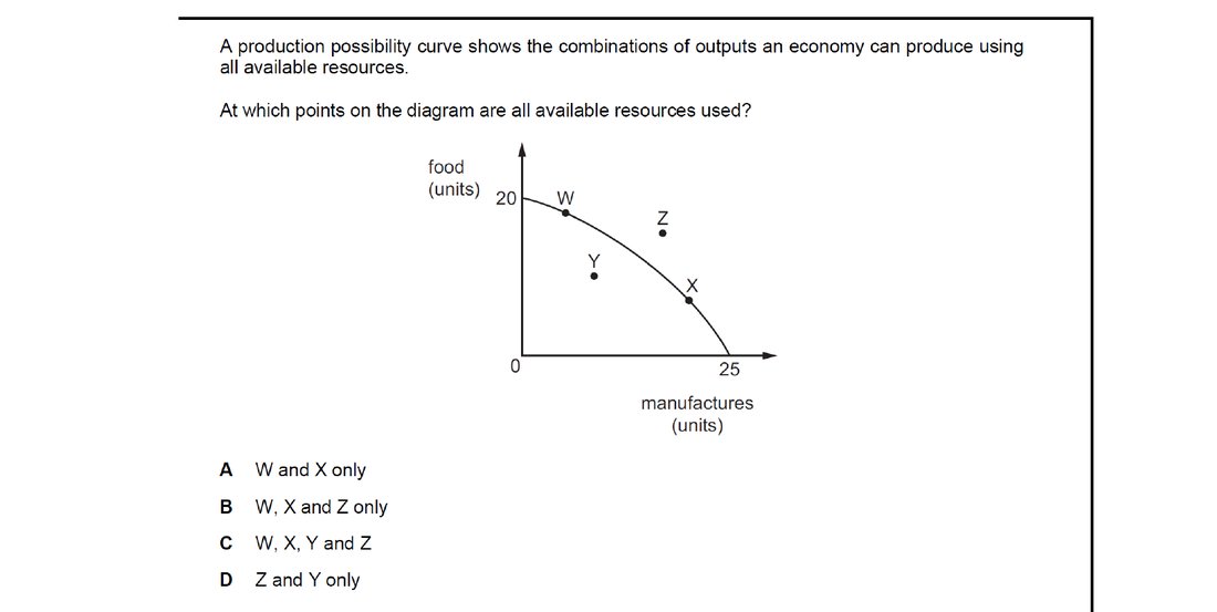
A PPC shows the maximum combinations of two goods producible when all resources are fully and efficiently used; any point on the curve uses all available resources, while points inside do not. Option A – W and X only – are the two on-curve points; Y lies inside (underuse of resources) and Z lies outside (unattainable). Hence only W and X represent full use.
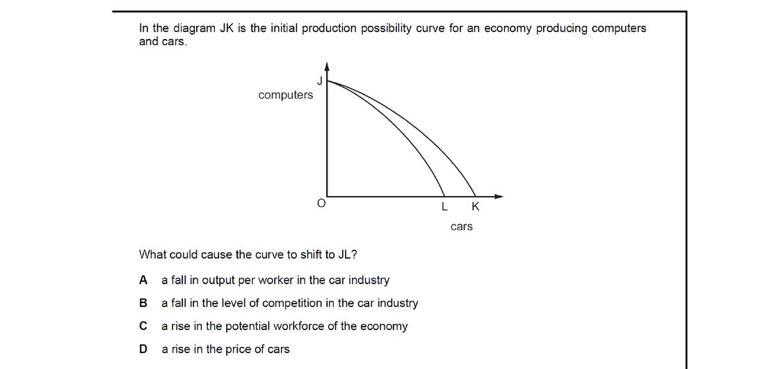
The new PPC JL has the same maximum output of computers (J unchanged) but a smaller maximum of cars (K to L). Only a fall in productivity in the car industry can reduce the maximum cars producible while leaving computer capacity untouched. Option A captures this. A bigger workforce (C) would expand the whole curve, the price of cars (D) shifts points along the curve, and competition (B) does not directly relocate the frontier.
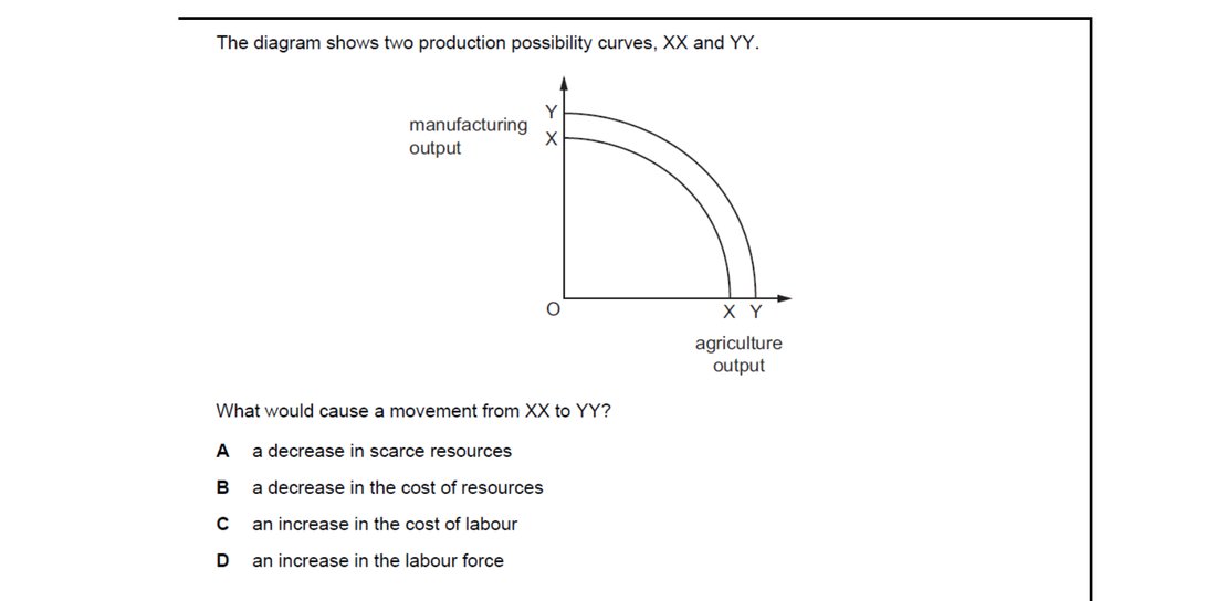
An outward shift of the PPC (XX to YY) requires more or better factors of production. Option D – an increase in the labour force – directly adds productive resources, raising the maximum output of both goods. A decrease in scarce resources (A) would shift the curve inwards, while changes in resource costs (B) and labour costs (C) affect prices and profits, not the productive frontier itself.
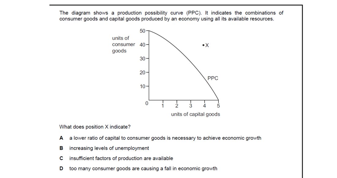
Position X lies outside the existing PPC, so it represents a combination of capital and consumer goods that is unattainable with current resources and technology. Option C – insufficient factors of production are available – states exactly this. Unemployment (B) and economic-growth claims (A, D) misread the position: more factors or better technology would have to shift the frontier outward to reach X.
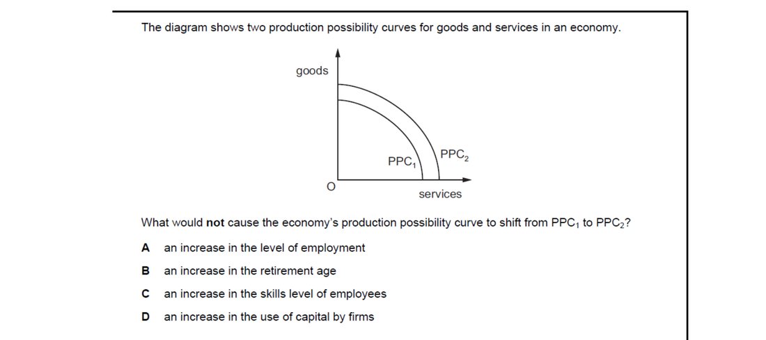
An outward shift of the PPC requires increases in the quantity or quality of factors, or in technology. Options B, C and D (later retirement, higher skills, more capital) all expand productive capacity. Option A – an increase in the level of employment – moves the economy towards or onto the existing PPC by using idle resources, but does not shift the frontier itself, so it is the correct 'not' answer.
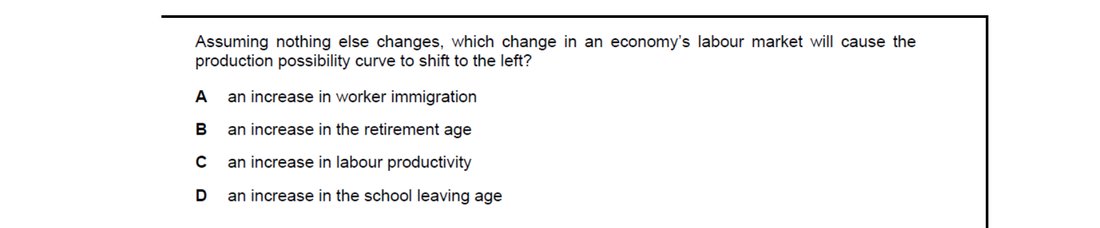
A leftward PPC shift means the economy can produce less of both goods, so the productive capacity of labour must fall. Option D – an increase in the school leaving age – temporarily removes young workers from the labour force, shrinking it. Immigration, a later retirement age and higher labour productivity (A, B, C) all expand productive capacity and would shift the PPC outwards, not inwards.
Attempt the practice questions above to build your score.
Self-evaluation checklist
After studying this chapter, you should be able to:
- Understand that a PPC shows the maximum level of output that an economy can achieve given current resources and state of technology.
- Explain why production is efficient at any point on the PPC.
- Explain why production at a point inside the PPC is inefficient and why production at a point outside the PPC cannot be achieved.
- Understand that PPCs that are convex to the origin indicate increasing opportunity costs.
- Analyse how shifts in the PPC, either inwards or outwards, show a change in productive capacity.
Want more practice? Drill this chapter's past-paper MCQs (82 questions) →